5 Quasi-isometries in Practice
Quasi-isometry of 1D MERA
In this section, we intuitively demonstrate how the tensor network graph of a 1D MERA is quasi-isometric to \(\mathbb H^2\). Below is a graphical representation of a 1D MERA:
- Isometry tensors are denoted by blue dots.
- Disentanger unitaries are denoted by orange.
- The graphical representation starts from 4 sites.
- The disentanglers are put on the same radius as the branching isometries.
Concretely, the MERA graph is specified as follows:
- At radius \(r\), there are \(\sim^{(8\cdot)} 2^r\) vertices in a regular polygon. The odd and even vertices correspond to isometries and disentanglers, respectively.
- Each disentangler at \(r\) is connected to two isometries at \(r+1\).
We next consider the behavior of geodesics in the 1D MERA. The highlighted paths are all geodesics from endpoints on the boundary.
The graph of the 1D MERA with disentanglers should be quasi-isometric to the graph below, after identifying the disentanglers with the isometries using local transformations (quasi-isometries only care about global properties). The geodesics in the following graph between two points at the same radius separated by angle \(\theta\) are determined by the following greedy rule:
- Connecting two points by an arc has distance \(\sim 2^r \theta\).
- Alternatively, we can reduce to \(r\mapsto r-1\) by extending the connecting path radially towards the center.
In particular, we see that the simplified graph captures:
- Exponential growth of the hyperbolic circumference w.r.t. the hyperbolic radius.
- Sideways connections by an angular arc (enabled by disentanglers).
The fundamental reason why a TTN (MERA without disentanglers) is not quasi-isometric to \(\mathbb H^2\) is that the tree structure only captures (1), but not (2). The metric for \(\mathbb H^2\) under \((\rho, \theta)\), where \(\rho\) is the hyperbolic radius, and \(\theta\) the angle, is \[ ds^2 = d\rho^2 + \sinh^2(\rho) d\theta^2 \xrightarrow{\rho \to \infty} d\rho^2 + \dfrac{e^{2\rho}}{4} d\theta^2 \] Both the \(d\rho\) and \(e^\rho \, d\theta\) terms are faithfully represented by the graph structure via the visual embedding below, so that the 1D MERA graph is quasi-isometric to \(\mathbb H^2\).
Cayley Graph of the Weeks Group
Recalling the Svarc-Milnor lemma, we have an explicit embedding of the Cayley graph of the fundamental group of the Weeks manifold into \(\mathbb H^3\) by the tiling generated by the fundamental domain .
We retrieved the Dirichlet domain and its associated face-pairing transformations from SnapPy.
- The Dirichlet domain is a canonical method for visualizing the fundamental domain of a manifold within its universal cover.
- The face-pairing transformations send the Dirichlet domain to its neighbors, effectively generating a regular tiling of \(\mathbb H^3\).
- The vertices of the Svarc-Milnor Cayley graph are the centers of the Dirichlet domains, with edges connecting vertices of neighboring domains.
- The Weeks Dirichlet domain has 26 vertices, 42 edges, and 18 faces. So the boundary grows approximately as \(18^r\).
- I only visualized the immediate neighbors of the center and the Cayley graph up to \(r=2\), to reduce clutter. Toggle the right-hand side to visualize specific components.
Hyperbolic Surfaces
The Poincaré ball model of \(\mathbb H^3\cong B_1(0)\) is equipped with the Riemmanian metric \[ ds^2 = \dfrac{4(dx^2 + dy^2 + dz^2)}{(1-r^2)^2}, \quad g_{ab} = \dfrac 4 {(1-r^2)^2} \begin{pmatrix} 1 & 0 & 0 \\ 0 & 1 & 0 \\ 0 & 0 & 1 \end{pmatrix} \]
Proposition 5.1 (Poincaré's and hyperbolic radius) The length \(\rho\) of a radial line which goes from \(r=0\) to \(r=R\) is \(\rho = 2\, \mathrm{arctanh}\, R\).
Proof: The radial scaling factor of length is \(2/(1-r^2)\). Integrating this yields \[ \rho = \int_0^R dr\, \dfrac{2}{1-r^2} = \log \dfrac{1+R}{1-R} = 2\, \mathrm{arctanh}\, R \]
Proposition 5.2 (hyperbolic sector area) The area \(A\) of the hyperbolic sector subtended by angle \(\phi\) and Poincaré radius \(R\in (0, 1)\) is \[ A = \dfrac{2\phi}{1/R^2 - 1} \]
Proof: The Jacobian of the inclusion map and the induced metric \(g'\) in \((\theta, r)\) coordinates are, respectively, \[\begin{align} J &= T\, \iota = \begin{pmatrix} \partial_{\theta }(r\cos\theta) & \partial_{\theta }(r\sin\theta) & 0 \\ \partial_{r} (r\cos\theta) & \partial_{r} (r\sin\theta) & 0 \end{pmatrix} = \begin{pmatrix} -r\sin\theta & r\cos\theta & 0 \\ \cos\theta & \sin\theta & 0 \end{pmatrix} \\ g' &= JgJ^T = \dfrac 4 {(1-r^2)^2} \begin{pmatrix} r^2 \\ & 1 \end{pmatrix}, \quad \sqrt{\det g'} = \dfrac{4r}{(1-r^2)^2} \end{align}\] Direct integration yields the desired area: \[\begin{align} A = \int_0^R \int_0^\phi \sqrt{\det g'} \, d\theta \, dr &= \phi \int_0^R \dfrac{4r}{(1-r^2)^2} \, dr = \phi \dfrac{2R^2}{1-R^2} = \dfrac{2\phi}{1/R^2 - 1} \end{align}\]
Proposition 5.3 (hyperbolic arc length) The length \(L\) of the arc subtended by angle \(\phi\) and Poincaré radius \(R\) is \[ L = \dfrac{2R\phi}{1-R^2} \]
Proof: The inclusion map \(\iota'\) of the curve has Jacobian \(J' = (-R\sin\theta, R\cos\theta, 0)\). The induced metric and length follows: \[ g'' = J' g (J')^T = \dfrac{4R^2}{(1-R^2)^2}, \quad \sqrt{\det g''} = \dfrac{2R}{1-R^2} \implies L = \dfrac{2R\phi}{1-R^2} \]
Proposition 5.4 (area law for hyperbolic spherical surfaces)
Consider a surface \(S\) on a hyperbolic sphere of radius \(\rho\in (0, \infty)\). Let \(A\) be the lateral area of the radial cone covering \(S\). We have \[ A = \tanh(\rho/2) |\partial S| \leq |\partial S| \]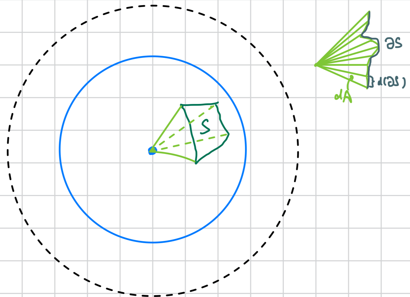
Figure 5.1: Hypothetical (for contradiction) constructions are in green. Geodesics are in blue.
Proof: Comparing propositions 5.2 and 5.3, we obtain \(A = RL\). Take the infinitesimal limit \((A, L)\mapsto (dA, d|\partial S|)\) and integrate to yield \(A = R|\partial S| = \tanh(\rho/2) |\partial S| \leq |\partial S|\).
Hypothesis 5.1 (area law for hyperbolic MERAs) For MERAs representing a Cayley graph generated by neighboring transformations per the Svarc-Milnor lemma, the area law is satisfied in the asymptotic limit of small lattices.
Proof: The area law follows from proposition 5.4 if the following two claims are true:
- Given a subsystem \(B\) of the lattice embedded on a hyperbolic sphere, the area (size) of the subsystem is faithfully represented by the hyperbolic area \(S\) as in proposition 5.4.
- The number of tensor legs crossing the lateral surface of the radial cone covering \(B\) is proportional to the lateral area \(A\) of the surface.
Note that the Cayley graph represents a regular tiling of \(\mathbb H^3\), so that in the small-tile limit:
- The hyperbolic area of a surface is approximated by the number of tiles
intersecting the surface up to constant factors.
- I’m imagining cubical volume elements in Euclidean space: the area of a surface is approximated by the number of cubical volume elements intersecting the surface.
- We can approximate the surface as a plane
in the small-tile limit, so the number of tile intersections is approximated
by the number of graph-edge cuts up to constant factors.
- In the Euclidean space, the intersection of a cubical volume element with a plane (assuming no intersection with vertices) cuts between \(3\) and \(4\) edges.
Combining the two observations, the number of tensor legs crossing the lateral surface and the radial patch are both proportional to the hyperbolic area of the surfaces.