8 f-Divergence

Key takeaways:

1. \(f\)-divergence is equivalent modulo \(c(t-1)\); convexity plus \(f(1)=f'(1)=1\) (which implies \(f\geq 0\)) implies locally \(\chi^2\).
2. Convexity of \(D_f\) 8.3 \(\iff\) DPI 8.2 \(\iff\) monotonicity 8.1 \(\iff\) convexity of \(f\).
3. There is no chain rule for \(f\)-divergences other than KL-divergence. Rényi divergence enjoys tensorization and chain rule (up to tilting); it includes KL, \(\chi^2\) and Hellinger as special cases. The Renyi chain rule does not imply the divergence chain rule, but \(\chi^2\) has a special chain rule (proposition 8.6).
4. TV as binary hypothesis testing: to reason about TV, break spaces into \(dP>dQ\) and \(dP<dQ\).
5. Several divergences are metrics (JS, \(H^2\)); one fast way to compare is to compare to metric, use triangle inequality, then use comparison inequality again.
6. TV does not enjoy tensorization properties; Hellinger divergence is both a metric and tensorizes well.
7. A powerful approximation theorem 8.4 reduces arbitrary spaces to finite ones. Similarly, the Harremoës-Vajda theorem 8.8 concludes the problem of joint range.

Locality and Fisher information:

1. Most \(f\)-divergences (with bounded \(f''\)) are locally \(\chi^2\): theorem 8.11 with respect to mixture interpolations.
2. Fisher information is only defined with respect to a family of distributions parameterized by \(\theta\).
   • It is the expectation of the Hessian of the log-pdf about \(\theta\): equation (8.6).
   • For regular families, \(\chi^2\) (mixture interpolations, in particular) is locally determined by the Fisher information 8.12.
3. Fisher information matrix is non-negative, monotonic, has its own chain rule 8.13 and variational characterization.

Definition

Definition 8.1 (f-divergence) Given a convex function \(f:(0, \infty)\to \mathbb R\) with \(f(1)=0\), for every two probability distributions over \(\mathcal X\), if \(P\ll Q\) then the \(f\) divergence is \[ D_f(P\|Q) = \mathbb E_Q \left[ f\left(\dfrac{dP}{dQ}\right) \right] \] Here \(f(0) = f(0_+)\) per limit. More generally, define \(f'(\infty) = \lim_{x\to 0^+} xf(1/x)\), we have \[ D_f(P\|Q) = \int_{q>0} q(x) f\left[ \dfrac{p(x)}{q(x)} \right] \, d\mu + f'(\infty) P[Q=0] \] this last generalization is needed to account for divergences like total variation. Intuitively, sums for terms with \(dQ=0\) are like \[ \int_{dQ=0} dQ f\left(\dfrac{dP}{dQ}\right) = \lim_{t=dP/dQ\to 0^+} \int \dfrac{dP}{t} f(1/t) \]

Examples of \(f\)-divergences:

1. KL-divergence: \(f(x)=x\log x\) to recover KL-divergence.
2. Total variation (TV): \(f(x) = \dfrac 1 2 |x - 1|\): \[ \mathrm{TV}(P, Q) = \dfrac 1 2 \mathbb E_Q \left|\dfrac{dP}{dQ} - 1\right| = \dfrac 1 2 \int |dP - dQ| = 1 - \int d(P\wedge Q) \] Recall that \(P\wedge Q\) is the pointwise minimum measure so \(\int d(P\wedge Q)\) is the overlap measure.
3. \(\chi^2\)-divergence: \(f(x)=(x-1)^2\). \[ \chi^2(P\|Q) = \mathbb E_Q \left(\dfrac{dP}{dQ} - 1\right)^2 = \int \dfrac{(dP - dQ)^2}{dQ} = \int \dfrac{dP^2}{dQ} + dQ - 2dP = \int \dfrac{dP^2}{dQ} - 1 \tag{8.1} \]
4. Squared Hellinger distance: \(f(x) = \left(1 - \sqrt x\right)^2\). \[ H^2(P, Q) = \int \left(\sqrt{dP} - \sqrt{dQ}\right)^2 = 2 - 2\int \sqrt{dPdQ} \tag{8.2} \] The quantity \(B(P, Q) = \int \sqrt{dPdQ}\) is the Bhattacharyya coefficient (Hellinger affinity). Note that \(H(P, Q) = \sqrt{H^2(P, Q)}\). The Hellinger distance is \(H(P, Q) = \sqrt{H^2(P, Q)}\).
5. Le Cam divergence: \(f(x) = \dfrac{1-x}{2x+2}\), \[ \mathrm{LC}(P, Q) = \dfrac 1 2 \int \dfrac{(dP - dQ)^2}{dP + dQ} \] The square root \(\sqrt{\mathrm{LC}(P, Q)}\), the Le Cam distance, is a metric.
6. Jensen-Shannon divergence take \(f(x) = x\log \dfrac{2x}{x+1} + \log \dfrac 2 {x+1}\). \[ \mathrm{JS}(P, Q) = D\left(P \| \dfrac{P+Q}{2}\right) + D\left(Q \| \dfrac{P+Q}{2}\right) \]

Proposition 8.1 \(\mathrm{TV}(P, Q) = \dfrac 1 2 \int |dP - dQ| = 1 - \int d(P\wedge Q)\).

Proof

Let \(E = \{x:dP > dQ\}\), then \[\begin{align} \int |dP - dQ| &= \int_E dP - d(P\wedge Q) + \int_{E^c} dQ - d(P\wedge Q) = \int_E dP + \int_{E^c} dQ - \int d(P\wedge Q) \\ &= \int_E dP + \int_{E^c} d(P\wedge Q)_{=dP} + \int_{E^c} dQ + \int_E d(P\wedge Q)_{=dQ} - 2\int d(P\wedge Q) \\ &= 2 - 2\int d(P\wedge Q) \end{align}\]

Proposition 8.2 The following quantities derived from divergences are metrics on the space of probability distributions \[ \mathrm{TV}(P, Q), \quad H(P, Q), \quad \sqrt{\mathrm{JS}(P, Q)}, \quad \sqrt{\mathrm{LC}(P, Q)} \]

Proposition 8.3 (closure properties)

1. \(D_f(Q \| P) = D_g(P \|Q)\) for \(g(x) = xf(1/x)\).
2. \(D_f(P\|Q)\) is a \(f\)-divergence, then \[ D_f(\lambda P + \bar \lambda Q \|Q), \quad D_f(P \| \lambda P + \bar \lambda Q), \quad \forall \lambda\in [0, 1] \] are \(f\)-divergences.
3. Linearity: \(D_{f+g} = D_f + D_g\).
4. Distinguishability: \(D_f(P \| P) = 0\)

Proof

For the first claim, \[ D_g(P \|Q) = \int dQ \left(\dfrac{dP}{dQ}\right) f\left(\dfrac{dQ}{dP}\right) = D_f(Q \| P) \] For the second claim, the other case can be obtained by using the equation above. \[ D_f(\lambda P + \bar \lambda Q \|Q) = \int dQ f\left(\lambda \dfrac{dP}{dQ} + \bar \lambda\right) \implies \tilde f(x) = f\left(\lambda x + \bar \lambda\right) \]

Proposition 8.4 (equivalence properties)

1. \(D_f(P\|Q) = 0\) for all \(P\neq Q\) iff \(f(x)=c(x-1)\) for some \(c\).
2. \(D_f = D_{f+c(x-1)}\); thus we can always assume \(f\geq 0\) and \(f'(1)=0\).

Proof

Claim \(1\) proceeds by computation (assuming continuity) \[ D_f(P \|Q) = c \int (dP / dQ - 1) dQ = 0 \] This means that \(c(x-1)\) is in the kernel of the linear operator \(f\mapsto D_f\). Pick \(c=-f'(1)\), then \(f(1)=f'(1)=0\); by convexity \(f\geq 0\).

Proposition 8.5 (special case of monotonicity) Joint divergence is unchanged through the same channel \[ D_f(P_XP_{Y|X} \| Q_XP_{Y|X}) = D_f(P_X \| Q_X) \] in particular, for the source-agnostic channel we have \[ D_f(P_XP_Y \| Q_XP_Y) = D_f(P_X \| Q_X) \]

Proof

Direct computation \[\begin{align} D_f(P_XP_{Y|X} \| Q_XP_{Y|X}) &= \int Q_X(x) dx \int P_{Y|X=x}(y)dy\, f\left[\dfrac{P_X(x) P_{Y|X=x}(y)}{Q_X(x) Q_{Y|X=x}(y)}\right]\\ &= \int Q_X(x) dx f\left(\dfrac{P_X(x)}{Q_X(x)}\right) = D_f(P_X \| Q_X) \end{align}\]

Information properties, MI

Theorem 8.1 (monotonicity) The joint is more distinguishable than the marginal: \[ D_f(P_{XY} \| Q_{XY}) \geq D_f(P_X \| Q_X) \] inequality is saturated when \(P_{Y|X} = Q_{Y|X}\).

Proof

Assume \(P_{XY} \ll Q_{XY}\), then expand and apply Jensen’s inequality \[\begin{align} D_f(P_{XY} \| Q_{XY}) &= \mathbb E_{X\sim Q_X} \mathbb E_{Y\sim Q_{Y|X}} f\left( \dfrac{dP_{Y|X} P_X}{dQ_{Y|X}Q_X} \right) \geq \mathbb E_{X\sim Q_X} f\left(\mathbb E_{Y\sim Q_{Y|X}} \dfrac{dP_{Y|X} P_X}{dQ_{Y|X}Q_X} \right) \\ &\geq \mathbb E_{X\sim Q_X} f\left( \dfrac{dP_X}{dQ_X} \right) = D_f(P_X \| Q_X) \end{align}\] To be more careful, on the first line we have \[\begin{align} \mathbb E_{Y\sim Q_{Y|X=x}} \dfrac{P_{Y|X=x}(y) P_X(x)}{Q_{Y|X=x}(y)Q_X(x)} &= \dfrac{P_X(x)}{Q_X(x)} \sum_y Q_{Y|X=x}(y) \dfrac{P_{Y|X=x}(y)}{Q_{Y|X=x}(y)} = \dfrac{P_X(x)}{Q_X(x)} \end{align}\] Inequality is saturated when, for every \(x\), \(P_{Y|X=x}=Q_{Y|X=x}\).

Definition 8.2 (conditional f-divergence) Given \(P_{Y|X}, Q_{Y|X}\) and \(P_X\), the conditional \(f\)-divergence is \[ D_f(P_{Y|X} \| Q_{Y|X} | P_X) = D_f(P_{Y|X} P_X \| Q_{Y|X} P_X) = \mathbb E_{x\sim P_X}\left[ D_f(P_{Y|X=x}\| Q_{Y|X=x}) \right] \]

Proof

The second statement requires some justification: \[\begin{align} D_f(P_{Y|X} P_X \| Q_{Y|X} P_X) &= \mathbb E_{x\sim P_X} \mathbb E_{y\sim Q_{Y|X=x}}\left[ f\left(\dfrac{P_{Y|X=x}(y)}{Q_{Y|X=x}(y)}\right) \right] \end{align}\]

Theorem 8.2 (data-processing inequality) Given a channel \(P_{Y|X}\) with two inputs \(P_X, Q_X\) \[ D_f(P_{Y|X} \circ P_X \| P_{Y|X} \circ Q_X) \leq D_f(P_X \| Q_X) \]

Proof

\(D_f(P_X \| Q_X) = D_f(P_{XY} \| Q_{XY}) \geq D_f(P_Y \| Q_Y)\), with two equalities given by proposition 8.5 and theorem 8.1. Inequality is saturated by the monotonicity condition \(P_{X|Y} = Q_{X|Y}\).

Theorem 8.3 (information properties of f-divergences)

1. Non-negativity: \(D_f(P\|Q) \geq 0\). If \(f\) is strictly convex at 1, i.e.  \[ \forall s, t\in [0, \infty), \alpha \in (0, 1) \text{ with } \alpha s + \bar \alpha t = 1: \quad \alpha f(s)+ \bar \alpha f(t) > f(1) = 0 \] then \(D_f(P\|Q) = 0 \iff P=Q\).
2. Conditional \(f\)-divergence; conditioning increases divergence: \(D_f(P_{Y|X} \circ P_X \| Q_{Y|X} \circ P_X) \leq D_f(P_{Y|X} \| Q_{Y|X} | Q_X) = D_f(P_{Y|X} P_X \| Q_{Y|X} P_X)\).
3. Joint-convexity: \((P, Q)\mapsto D_f(P\|Q)\) is jointly convex; consequently, \(P\mapsto D_f(P\|Q)\) and \(Q\mapsto D_f(P\|Q)\) are also convex.

Proof

For non-negativity, apply monotonicity to \[ D_f(P_X \| P_Y) = D_f(P_{X, 1} \| P_{Y, 1}) \geq D_f(1 \| 1) = 0 \] Assume \(P\neq Q\) so there exists measurable \(A\) such that \(P[A]=p \neq Q[A] = Q\), then apply the \(\chi_A\) channel and apply DPI; both cases \(q=1\) and \(q\neq 1\) contradict strict convexity. Claim (2) follows from monotonicity and recognize \(P_{Y|x}\circ P_X\) as the marginal of \(P_{Y|X}P_X\). Joint convexity follows from standard latent variable argument: to prove joint convexity \[ D(\lambda P_0 + \bar \lambda P_1 \| Q_0 + \bar \lambda Q_1) \leq \lambda D(P_0 \| Q_0) + \bar \lambda D(P_1 \| Q_1) \] Take \(\theta \sim \mathrm{Ber}_\lambda \to (P, Q)\), then the RHS is \(D(P_{P|\lambda} \| P_{Q|\lambda} | P_\lambda)\) while the LHS is \(D(P_{P|\lambda}\circ P_\lambda\| P_{Q|\lambda} \circ P_\lambda)\)

The following powerful theorem allows us to reduce any general problem to finite alphabets.

Theorem 8.4 (finite approximation theorem) Given two probability measures \(P, Q\) on \(\mathcal X\) with \(\sigma\)-algebra \(\mathcal F\). Given a finite \(\mathcal F\)-measurable partition \(\mathcal E = \{E_1, \cdots, E_n\}\), define the distribution \(P_{\mathcal E}\) on \([n]\) by \(P_{\mathcal E}(j) = P[E_j]\), similarly for \(Q\), then \[ D_f(P\|Q) = \sup_{\mathcal E} D_f(P_{\mathcal E} \| Q_{\mathcal E}) \] where \(\sup\) is over all finite \(\mathcal F\)-measurable partitions.

We omit the technical proof above.

Definition 8.3 (f-information) The \(f\)-information is defined by \[ I_f(X; Y) = D_f(P_{XY} | P_XP_Y) \]

Definition 8.4 (f-DPI) For \(U\to X\to Y\), we have \(I_f(U; Y) \leq I_f(U; X)\).

Proof: \(I_f(U; X) = D_f(P_{UX} \|P_UP_X) \geq D_f(P_{UY} \| P_UP_Y) = I_f(U; Y)\).

Proposition 8.6 (χ² chain rule) \(\chi^2(P_{AB} \| Q_{AB}) = \chi^2(P_B \| Q_B) + \mathbb E_{Q_B} \left[ \chi^2(P_{A|b} \| Q_{A|b}) \dfrac{P_B^2}{Q_B^2} \right]\)

Proof

Invoke equation (8.1): \[\begin{align} \chi^2 (P_{AB} \| Q_{AB}) &= \mathbb E_P \left[ \dfrac{P_{AB}^2}{Q_{AB}^2} \right] - 1 = \mathbb E\dfrac{P_B^2}{Q_B^2} - 1 + \mathbb E\left[ \dfrac{P_B^2}{Q_B^2} \left( \dfrac{P_{A|B}^2}{Q_{A|B}^2} - 1 \right) \right] \\ &= \chi^2(P_B \| Q_B) + \mathbb E_{P_B} \left[\chi^2(P_{A|B} \| Q_{A|B}) \left(\dfrac{P_B^2}{Q_B^2}\right)^2\right] \end{align}\]

TV and Hellinger, hypothesis testing

In a binary hypothesis testing problem, one is given an observation \(X\), which is known to be \(X\sim P\) or \(X\sim Q\). The goal is to decide \(\lambda\in \{0, 1\}\) based on \(X\). In other words, \[ \lambda \to X\to \hat \lambda \] Our objective is to find a possibly randomized decision function \(\phi:\mathcal X\to \{0, 1\}\) such that \[ P[\phi(X)=1] + Q[\phi(X) = 0] \] is minimized. We will see that optimization leads to TV, while asymptotic tensorization leads to \(H^2\).

Theorem 8.5 (variational characterizations of TV)

1. \(\sup\)-representation: let \(\mathcal F = \{f:\mathcal X\to \mathbb R, \|f\|_\infty \leq 1\}\), then \[ \mathrm{TV}(P, Q) = \sup_E P(E) - Q(E) = \dfrac 1 2 \sup_{f\in \mathcal F} \left[\mathbb E_P f(X) - \mathbb E_Q f(X)\right] \] Supremum is achieved by \(f=\chi_E\), where \(E=\{x:p(x)>q(x)\}\).
2. \(\inf\)-representation: Provided the diagonal is measurable, \[ \mathrm{TV}(P, Q) = \min_{P_{XY}} \{P_{XY}[X\neq Y] \text{ subject to } P_X=P, P_Y=Q\} \]

Proof

The upper bound by \(\mathrm{TV}\) is intuitive; to demonstrate saturation, let \(E = \{x:p(x)>q(x)\}\), then \[\begin{align} 0 = \int [p(x) - q(x)]\, d\mu &= \int_E + \int_{E^c} [p(x) - q(x)]\, d\mu \\ \int_E [q(x) - p(x)]\, d\mu &= \int_{E^c} [p(x) - q(x)]\, d\mu \end{align}\] The sum of these two integrals (note the definition of \(E\)) equals \(2\mathrm{TV}\), then \[ \mathrm{TV}(P, Q) = \dfrac 1 2 \int \chi_E[(q(x) - p(x)]\, d\mu = \dfrac 1 2 \mathbb E_P \chi_E(X) - \mathbb E_Q \chi_E(X) \] For the \(\inf\) representation, given any coupling \(P_{XY}\), for \(f\in \mathcal F\) we have \[ \mathbb E_P f(X) - \mathbb E_Q f(X) = \mathbb E_{P_{XY}}[f(X) - f(Y)] \leq 2 P_{XY}[X\neq Y] \] This shows that the \(\inf\)-representation is always an upper bound; we obtain saturation when \(X\neq Y\) only happens for possible values of \(X\) disjoint from possible values of \(Y\), and \(f\) is the indicator function on the disjoint support. This is satisfied by the following construction given \(P, Q\):

1. Let \(\pi = \int \pi(x)\, d\mu\) denote the overlap scalar, where \(\pi(x) = \min(p(x), q(x))\).
2. With probability \(\pi\) take \(X=Y\) sampled from the overlap density \[ r(x) = \dfrac 1 \pi \pi(x) \]
3. With probability \(1-\pi\) sample \(X, Y\) independently from \[ p_1(x) = \dfrac{p(x) - \pi(x)} {1 - \pi}, \quad q_1(x)=\dfrac{q(x) - \pi(x)}{1 - \pi} \]
   

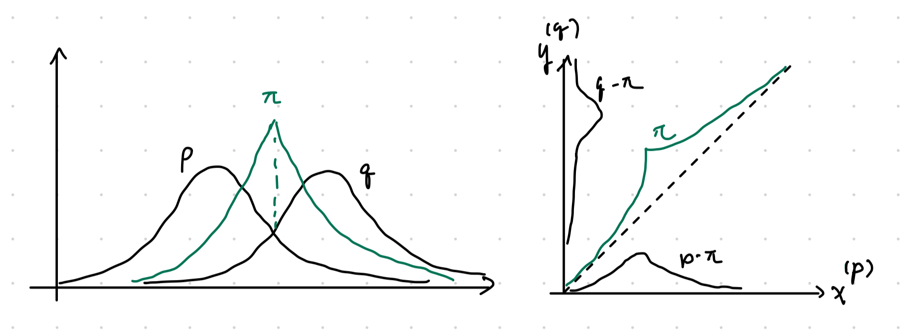
   Figure 8.1: Visual representation of joint construction.

Note that \(p_1, q_1\) have disjoint supports. Now, the marginals are indeed \(P, Q\), and this saturates the inequality since \(P_{XY}[X\neq Y] = 1-\pi=\mathrm{TV}(P, Q)\)

The total variation distance does not tensorize well, but we have the following sandwich bound: \[ \dfrac 1 2 H^2 \leq \mathrm{TV}\leq H\sqrt{1 - \dfrac{H^2}{4}} \leq 1 \tag{8.3} \]
We also have the following asymptotic theorem:

Theorem 8.6 (asymptotic equivalence of TV and Hellinger) For any sequence of distributions \(P_n, Q_n\) \[\begin{align} \mathrm{TV}(P_n^{\otimes n}, Q_n^{\otimes n}) \to 0 &\iff H^2(P_n, Q_n) = o(1/n) \\ \mathrm{TV}(P_n^{\otimes n}, Q_n^{\otimes n}) \to 1 &\iff H^2(P_n, Q_n) = \omega(1/n) \end{align}\] Recall that \(o(1/n)\) means asymptotically smaller growth than \(1/n\), while \(\omega(1/n)\) is the opposite.

Proof

We will need the following tensorization result from corollary 8.2: \[ H^2_n = 2 - 2\left(1 - \dfrac 1 2 H^2_1\right)^n \approx 2 - 2\exp\left[-n\left(1 - \dfrac 1 2 H^2_1\right)\right] \] Using the sandwich bound (8.3), \(\mathrm{TV}\to 0\) implies the exponential going to \(0\), then \(H^2_1\) has to grow slower than \(1/n\). The oppose is true for \(\mathrm{TV}\to 1\).

Joint range

We first provide a special case of an inequality.

Theorem 8.7 (Pinsker's inequality) For any two distributions, \(D(P\|Q) \geq (2\log e) \mathrm{TV}(P, Q)^2\)

Proof

By DPI, it suffices to consider Bernoulli distributions via the channel \(1_E\) which results in Bernoulli with parameter \(P(E)\) or \(Q(E)\). Working in natural units, Pinsker’s inequality for Bernoulli distributions yield \[ \sqrt{\dfrac 1 2 D(P\|Q)} \geq \mathrm{TV}(1_E\circ P, Q_E\circ Q) = |P(E) - Q(E)| \] Taking supremum over all \(E\) yields the desired inequality per the TV variational characterization theorem 8.5.

Definition 8.5 (joint range) Given two \(f\)-divergences \(D_f\) and \(D_g\), their joint range \(\mathcal R\subset [0, \infty]^2\) is defined by \[ \mathcal R = \mathrm{Image}\left[ (P, Q)\mapsto (D_f(P\|Q, D_g(P\|Q)) \right] \] The joint range over \(k\)-ary distribution is denoted \(\mathcal R_k\).

Our next result will characterize the set of \(f\)-divergences.

Lemma 8.1 (Fenchel-Eggleston-Carathéodory theorem) Let \(S\subset \mathbb R^d\) and \(x\in \mathrm{co}(S)\). There exists a set of \(d+1\) points \(S'=\{x_1, \cdots x_{d+1}\}\in S\) such that \(x\in \mathrm{co}(S')\). If \(S\) has at most \(d\) connected components, then \(d\) points are enough.

As a corollary of the following theorem, it suffices to prove joint range for Bernouli, then convexify the range.

Theorem 8.8 (Harremoës-Vajda) \(\mathcal R = \mathrm{co}(\mathcal R_2) = \mathcal R_4\) where \(\mathrm{co}\) denotes the convex hull with a natural extension of convex operations to \([0, \infty]^2\). In particular,

1. \(\mathrm{co}(\mathcal R_2) \subset\mathcal R_4\): standard latent variable argument.
2. \(\mathcal R_k \subset \mathrm{co}(\mathcal R_2) = \mathcal R_4\).
3. \(\mathcal R = \mathcal R_4\): the approximation theorem already implies \(\mathcal R = \overline{\bigcup_k \mathcal R_k}\); the closure is technical.

Proof

First consider claim \(1\). Construct a convex divergence as follows: for two pairs of distributions \((P_0, Q_0)\) and \((P_1, Q_1)\) on \(\mathcal X\) and \(\lambda \in [0, 1]\). Define the typical Bernoulli latent joint \((X, B)\) by \(P_B = Q_B = \mathrm{Ber}(\alpha)\) and \((P, Q)_{X|B=j} = (P_j, Q_j)\). Applying the conditional divergence to obtain \[ D_f(P_{XB} \| Q_{XB}) = \bar \alpha D_f(P_0\|Q_0) + \alpha D_f(P_1 \| Q_1) \implies \mathrm{co}(\mathcal R_2)\subset \mathcal R_4 \] Onto the most nontrivial claim \(2\): fixing \(k\) and distributions \(P, Q\) on \([k]\) with distributions \((p_j), (q_j)\), w.l.o.g. make \(q_{j>1}>0\) and concentrate \(q_1=0\) (i.e. concentrate all empty points onto \(j=1\). Consider the equivalence class \(\mathcal S\) of all \((\tilde p_j, \tilde q_j)\) which have the same likelihood ratio on the support of \(q\): Let \(\phi_{j>1} = p_j / q_j\) and consider \[ \mathcal S = \left\{ \tilde Q = (\tilde q_j)_{j\in [k]}: \tilde q_j\geq 0, \sum \tilde q_j=1, \tilde q_1=0, \right\} \] Note that \(\mathcal S\) it the intersection of

1. The simplex of all distributions \(\tilde q\).
2. The half-space specified by \(\tilde q\cdot \phi \leq 1\).

We can next identify the boundary of \(\mathcal S_e\subset \mathcal S\):

1. \(\tilde q_{j\geq 2}=1\) and \(\phi_j\leq 1\).
2. \(\tilde q_{j_1}+\tilde q_{j_2}=1\) and \(\tilde q_{j_1}\phi_{j_1} + \tilde q_{j_2}\phi_{j_2}=1\).

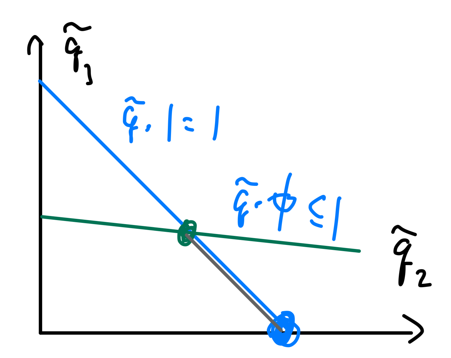
Figure 8.2: Gray line corresponds to \(S\); blue and green dots correspond to elements of \(S_e\) identified by (1) and (2), respectively.

We next have \(\mathcal S = \mathrm{co}(\mathcal S_e)\); so for \(Q\), there exists extreme points \(\tilde Q_j\in \mathcal S_e\) (note that \(\mathcal S_e\) is dependent upon \(Q\)!) with support on at most \(2\) atoms (binary distributions) such that \(Q = \alpha_j \tilde Q_j\). The map asspciating \(\tilde P\) given \(\tilde Q\) is \[ \tilde p_j = \begin{cases} \phi_j \tilde q_j & j\in \{2, \cdots, k\}, \\ 1 - \sum_{j=2}^k \phi_j \tilde q_j & j = 1 \end{cases} \] On this particular set which fixes the likelihood ratio, the divergence is an affine map: \[ \tilde Q \mapsto D_f(\tilde P \| \tilde Q) = \sum_{j\geq 2}\tilde q_j f(\phi_j) + f'(\infty)\tilde p_1 \implies D_f(P\|Q) = \sum_{j=1}^m \alpha_i D_f(\tilde P_i \|\tilde Q_i) \]

We defer detailed examples of joint ranges to the book (7.6).

Rényi divergence

The Rényi divergences are a monotone transformation of \(f\)-divergences; they satisfy DPI and other properties.

Definition 8.6 (Rényi divergence) For \(\lambda\in \mathbb R- \{0, 1\}\), the Rényi divergence of order \(\lambda\) between distributions \(P, Q\) is \[ D_\lambda(P \| Q) = \dfrac 1 {\lambda - 1} \log \mathbb E_Q \left[ \left(\dfrac{dP}{dQ}\right)^\lambda \right] \]

To see its connection with entropy, note that \[ \mathbb E_Q \left(\dfrac{dP}{dQ}\right)^\lambda = \mathrm{sgn}(\lambda - 1) D_f(P\|Q) + 1, \quad f = \mathrm{sgn}(\lambda - 1)(x^\lambda - 1) \] with which the Rényi entropy becomes (the \(\mathrm{sgn}(\lambda - 1)\) is just there to keep \(f\) convex): \[ D_\lambda(P\|Q) = \dfrac 1 {\lambda - 1} \log \left[1 + \mathrm{sgn}(\lambda - 1) D_f(P\|Q) \right], \quad f = \mathrm{sgn}(\lambda - 1)(x^\lambda - 1) \tag{8.4} \]

Proposition 8.7 Under regularity conditions, \[ \lim_{\lambda \to 1} D_\lambda (P \|Q) = D(P \| Q) \]

Proof

Expand \((d_QP)^\lambda = \exp(\lambda \ln d_QP)\) about \(\lambda=1\): \[ (d_QP)^{\lambda} \approx d_QP + \ln d_QP \cdot d_QP \cdot (\lambda - 1) \] Taking \(\mathbb E_Q\) yields \(1 + (\lambda - 1)\mathbb E_P[\ln d_QP]\); then substituting into \(\log x \approx 1+x\) yields \[ D_{\lambda_\to 1}(P \| Q) = \dfrac 1 {\lambda - 1} \log \left[ 1 + (\lambda - 1)\mathbb E_P[\ln d_QP] \right] = \mathbb E_P \ln d_QP = D(P \| Q) \]

Proposition 8.8 (special cases of Rényi divergence) Consider \(\lambda = 1/2, 2\): \[ D_2 = \log(1 + \chi^2), \quad D_{1/2} = -2\log\left(1 - \dfrac{H^2}{2}\right) \]

Proof

The \(D_2\) case is apparant in light of equation (8.4). Substitute \(\lambda = 1/2\): \[ D_{1/2} = \dfrac 1 {1/2 - 1} \log[1 - D_{x\mapsto 1 - \sqrt x}(P\|Q)] \] It remains to show that \(D_{1 - \sqrt x} (P\|Q) = \dfrac{H^2}{2}\), applying equation (8.2) \[ \mathbb E_Q\left[1 - \sqrt{d_QP}\right] = \dfrac 1 2 \mathbb E_Q \left(1 - \sqrt{d_QP}\right)^2 = 1 - \int \sqrt{dPdQ} \]

Several other properties:

1. \(\lambda \mapsto D_\lambda D(P\|Q)\) is non-decreasing and \(\lambda \mapsto (1 - \lambda) D_\lambda(P\|Q)\) is concave.
2. For \(\lambda \in [0, 1]\) the divergence \(D_\lambda\) is jointly convex.
3. The Rényi entropy for finite alphabet is \(H_\lambda(P) = \log m - D_\lambda(P \| U)\).

Definition 8.7 (conditional Rényi entropy) Given \(P_{X|Y}, Q_{X|Y}\) and \(P_Y\) \[\begin{align} D_\lambda(P_{X|Y} \| Q_{X|Y} | P_Y) &= D_\lambda(P_{X|Y} P_Y \| Q_{X|Y} P_Y) = \dfrac 1 {\lambda - 1} \log \mathbb E_{Q_{X|Y}P_Y} \left[ \dfrac{(P_{X|Y}P_Y)(X, Y)}{(Q_{X|Y}P_Y)(X, Y)} \right]^\lambda \\ &= \dfrac 1 {\lambda - 1} \log \mathbb E_{y\sim P_Y} \int_{\mathcal X} P_{X|Y=y}(x)^\lambda Q_{X|Y=y}(x)^{1-\lambda} \end{align}\]

Proposition 8.9 (Rényi chain rule) Given \(P_{AB}, Q_{AB}\), define the \(\lambda\)-tilting of \(P_B\) towards \(Q_B\) by \[ P_B^{(\lambda)}(b) = P_B^\lambda(b) Q_B^{1-\lambda}(b) \exp \left[ -(\lambda - 1) D_\lambda(P_B \| Q_B) \right] \] joint Rényi divergence decomposes as \[ D_\lambda(P_{AB} \| Q_{AB}) = D_\lambda(P_B \| Q_B) + D_\lambda( P_{A|B} \| Q_{A|B} | P_B^{(\lambda)}) \]

Proof

First need to prove that \(P_B^{(\lambda)}\) is indeed correctly normalized: \[\begin{align} \exp \left[ -(\lambda - 1) D_\lambda(P_B \| Q_B) \right] &= \mathbb E_Q \left[\left(\dfrac{dP}{dQ}\right)^\lambda\right] = \int P_B^\lambda(b) Q_B^{1-\lambda}(b)\, db \end{align}\] Next up, computing the RHS explicitly, we have \[\begin{align} (\lambda - 1) [D_\lambda(P_B \| Q_B) + D_\lambda( P_{A|B} \| Q_{A|B} | P_B^{(\lambda)})] &= \log \int_{\mathcal B} \left[ P_B(b)^\lambda Q_B(b)^{1-\lambda} \cdot \int_{\mathcal A} P_{A|B=b}(a)^\lambda Q_{A|B=b}(a)^{1-\lambda} \right] \\ &= \log \mathbb E_{Q_{AB}} \left(\dfrac{dP_{AB}}{dQ_{AB}}\right)^\lambda = D_\lambda(P_{AB} \| Q_{AB}) \end{align}\]

Corollary 8.1 (Rényi tensorization) Specializing the chain rule to independent joints, \[ D_\lambda \left(\prod P_{X_j} \| \prod Q_{X_j}\right) = \sum_j D_\lambda(P_{X_j} \| Q_{X_j}) \]

Corollary 8.2 (tensorization of χ² and Hellinger) Applying tensorization and proposition 8.8: \[\begin{align} 1 + \chi^2 \left(\prod_j P_j \| \prod_j Q_j\right) &= \prod_j 1 + \chi^2(P_j \| Q_j) \\ 1 - \dfrac 1 2 H^2 \left(\prod P_j, \prod Q_j\right) &= \prod_j 1 - \dfrac 1 2 H^2(P_j, Q_j) \end{align}\]

Proposition 8.10 (variational characterization via KL) Show that \(\forall \alpha \in \mathbb R\): \[ \bar \alpha D_\alpha(P \|Q) = \inf_R \left[ \alpha D(R\|P) + \bar \alpha D(R\|Q) \right] \]

Proof

The KL case \(\alpha=1\) holds trivially with \(R=P\). otherwise expand the LHS to \[\begin{align} \bar \alpha D_\alpha(P\|Q) &= -\log \mathbb E_Q \left(\dfrac{dP}{DQ}\right)^\alpha = \log \mathbb E_Q \left( \dfrac{dQ}{dP} \right)^\alpha \end{align}\] Expand the RHS to \[\begin{align} \alpha D(R\|P) + \bar \alpha D(R\|Q) &= \mathbb E_R \log \left[ \left(\dfrac{dR}{dP}\right)^\alpha \left(\dfrac{dR}{dQ}\right)^{\bar \alpha} \right] = \mathbb E_R \log \dfrac{dR}{dP^\alpha dQ^{\bar \alpha}} \\ &= \mathbb E_R \log \dfrac{dR}{dQ} \cdot \left(\dfrac{dQ}{dP}\right)^\alpha = D(R \| Q) + \mathbb E_R \log \left(\dfrac{dQ}{dP}\right)^\alpha \end{align}\] We wish to establish the bound \[\begin{align} \log \mathbb E_Q \left( \dfrac{dQ}{dP} \right)^\alpha \leq \mathbb E_R \log \left[ \dfrac{dR}{dP^\alpha dQ^{\bar \alpha}} \right] &= D(R \| Q) + \mathbb E_R \log \left(\dfrac{dQ}{dP}\right)^\alpha \\ D(R\|Q) &\geq \mathbb E_R \log \left(\dfrac{dP}{dQ}\right)^\alpha - \log \mathbb E_Q \left(\dfrac{dP}{dQ}\right)^\alpha \end{align}\] Comparison between \(\log \mathbb E\) and \(\mathbb E\log\) screams Donsker-Varadhan 5.5: \[ D(R \|Q) \geq \mathbb E_R f - \log \mathbb E_Q \exp f \] for \(f = \alpha \log(dP/dQ)\) being the likelihood ratio. Recall that the saturation constraint is \[ \log \left(\dfrac{dP}{dQ}\right)^\alpha = f = \log \dfrac{dR}{dQ} + C \iff \dfrac{P(x)^\alpha}{Q(x)^\alpha} = \dfrac{R(x)}{Q(x)} \iff dR \propto dP^\alpha dQ^{\bar \alpha} \] the proportionality freedom comes from invariance of \(f\mapsto f+C\) in Donsker-Varadhan and is determined by the normalization constraint. The final result is simply the Renyi-tilt of \(P\) towards \(Q\) given by \[ R(x) = P(x)^\alpha Q(x)^{\bar \alpha} \exp \left[ -\bar \alpha D_\alpha(P \| Q) \right] \]

Variational characterizations

Given a convex function \(f:(0, \infty)\to \mathbb R\), recall that is convex conjugate \(f^*:\mathbb R\to \mathbb R\cup \{+\infty\}\) is defined by \[ f^*(y) = \sup_{x\in \mathbb R_+} xy - f(x) \] For a differentiable convex function, \(\mathrm{dom}(f^*) = \{y: f^*(y)<\infty\}\) is the range of \(\nabla f\). The Legendre transform is convex, involutary, and satisfies \[ f(x) + f^*(y) \geq xy \] Similarly, the convex conjugate of any convex functional \(\Psi(P)\) is, under suitable technical conditions \[ \Psi^*(g) = \sup_P \int g\, dP - \Psi(P), \quad \Psi(P) = \sup_g \int g\, dP - \Psi^*(g) \] When \(P\) is a probability measure, \(\int g\, dP = \mathbb E_P[g]\). In this section, we identify \(f:(0, \infty)\to \mathbb R\) with its convex extension \(f:\mathbb R\to \mathbb R\cup \{+\infty\}\) (one can just take \(f = \infty\) for all inputs outside the original domain); different choices of \(f\)’s extension yield different variational formulas:

Theorem 8.9 (supremum characterization of f-divergences) Given probability measures \(P, Q\) on \(\mathcal X\); fix an extension of \(f\) and corresponding Legendre transform \(f^*\); denote \(\mathrm{dom}(f^*) = (f^*)^{-1}(\mathbb R)\), then \[ D_f(P\|Q) = \sup_{g:\mathcal X\to \mathrm{dom}(f^*)} \mathbb E_P[g(X)] - \mathbb E_Q[(f^*\circ g)(X)] \]

As a result of this variational characterization, we obtain:

1. Joint convexity: \((P, Q)\mapsto D_f(P\|Q)\) is convex since \(D_f\) is a supremum of affine functions.
2. Weak lower semicontinuity: a simple counter-example to continuity is \(\sum_{j=1}^n X_j/\sqrt n\to \mathcal N(0, 1)\) for \(X_j=2\mathrm{Ber}(1/2)-1\) but each partial sum remains discrete. By the same line of reasining in theorem 5.6:
   \[ \liminf_{n\to \infty} D_f(P_n\|Q_n) \geq D_f(P\|Q) \]
3. Relation to DPI: again, variational characterizations can be used as a version of DPI when using \(1_E\) since it allows one to bound the event variation using \(f\)-divergence.

Example 8.1 (TV) Recall, for \(\mathrm{TV}, f(x)=|x-1|/2\); extending as such to \(\mathbb R\) to obtain the conjugate \[ f^*(y) = \sup_x xy - \dfrac 1 2 |x-1| = \begin{cases} \infty & |y|>1/2 \\ y & |y| \leq 1/2 \end{cases} \] Applying theorem 8.9 recovers theorem 8.5: \[ \mathrm{TV}(P, Q) = \sup_{g(x)\in [-1/2, 1/2]} \mathbb E_P[g] - \mathbb E_Q[g] \]

Example 8.2 (Hellinger) The conjugate for Hellinger \(f(x) = (1-\sqrt x)^2\) is \(f^*(y) = \frac 1 {1-y} - 1\) with \(y\in (-\infty, 1)\), yielding \[\begin{align} H^2(P, Q) &= \sup_{g(x)\in (-\infty, 1)} \mathbb E_P[g] - \mathbb E_Q\left[\dfrac 1 {1-g} - 1\right]\\ &= \sup_{g> 0} \mathbb E_P[1-g] - \mathbb E_Q \dfrac 1 g + 1 = 2 - \inf_{g> 0} \mathbb E_P g + \mathbb E_Q \dfrac 1 g \end{align}\] Given \(f:\mathcal X\to [0, 1]\) and \(\tau \in (0, 1)\), we have \(h=1-\tau f\) and \(\frac 1 h \leq 1 + \frac{\tau}{1-\tau} f\), then \[ \mathbb E_P[f] \leq \dfrac 1 {1-\tau} \mathbb E_Q f + \dfrac 1 \tau H^2(P, Q), \quad \forall f:\mathcal X\to [0, 1], \quad \tau \in (0, 1) \] Note that for this inequality we don’t need \(h\) to saturate the \(\inf h>0\) condition: only a subset suffices.

Proposition 8.11 (χ²-divergence) Given \(\chi^2\) and \(f(x)=(x-1)^2\), the conjugate is \(f^*(y) = y + \frac{y^2}{4}\) and \[\begin{align} \chi^2(P\|Q) &= \sup_{g:\mathcal X\to \mathbb R} \mathbb E_P g - \mathbb E_Q \left[ g + \dfrac{g^2}{4} \right] \\ &= \sup_{g:\mathcal X\to \mathbb R} \sup_{\lambda \in \mathbb R} \left[ \mathbb E_P g - \mathbb E_Q g \right] \lambda - \dfrac{\mathbb E_Q[g^2]}{4} \lambda^2 \end{align}\] Complete the square in the inner problem to obtain \[\begin{align} -a \lambda^2 + b\lambda &= -a\left(\lambda - \dfrac b {2a}\right)^2 + \dfrac{b^2}{4a} \implies \chi^2(P\|Q) = \sup_{g:\mathcal X\to \mathbb R} \dfrac{\left(\mathbb E_P g - \mathbb E_Q g\right)^2}{\mathbb E_Q[g^2]} \end{align}\] The choice of \(g\) is invariant under \(g\mapsto g+c\), so we obtain \[ \chi^2(P\|Q) = \sup_{g:\mathcal X\to \mathbb R} \dfrac{\left(\mathbb E_P g - \mathbb E_Q g\right)^2}{\mathrm{Var}_Q[g^2]} \tag{8.5} \] Given two hypotheses \(P, Q\), \(\chi^2\) is the maximum ratio between the squared-distance between the mean statistic \(g\) and its variance under \(Q\).

Example 8.3 (Jenson-Shannon divergence) For JS we have \(f(x) = x\log \dfrac{2x}{1+x} + \log \dfrac{2}{1+x}\) with conjugate and variational characterization \[\begin{align} f^*(s) &= -\log(2 - e^s), \quad s\in (-\infty, \log 2) \\ \mathrm{JS}(P, Q) &= \sup_{g(x)<\log 2} \mathbb E_P g + \mathbb E_Q \log(2 - e^g) \end{align}\] Reparameterize with \(h=e^g/2\) to obtain \[ \mathrm{JS}(P, Q) = \log 2 + \sup_{h(x)\in (0, 1)} \mathbb E_P \log h + \mathbb E_Q\log(1-h) \] In desity estimation, suppose \(P\) is the data distribution wish to approximate with \(P_{f_\theta(Z)}\), then we have \[ \inf_\theta \sup_\phi \mathbb E_{X\sim P} [\log h_\phi(X)] + \mathbb E_{Z\sim \mathcal N} \log[1 - h_\phi(f_\theta(Z))] \] Here \(f_\theta\) is the generator, and \(h_\phi\) is the critic in GAN.

Proposition 8.12 (KL) We have \(f(x\geq 0) = x\log x\). Extend to \(f(x<0) = \infty\); the convex conjugate is (in natural units) \(f^*(y) = e^y/e\) thus \[ D(P\|Q) = \sup_{g:\mathcal X\to R} \mathbb E_P[g] - \mathbb E_Q[e^g] + 1 \] Do the substitution \(g\mapsto g+c\) to obtain the following expression, and solve for the analytic optimal \(c\). Fixing \(g\), let \(\alpha = \mathbb E_Q[e^g]\) be a constant. The extremal value of \(c - a\cdot e^c\) is obtained at \(c=-\ln a\) as \(-\ln a - 1\), yielding \[ D(P\|Q) = \sup_{g:\mathcal X\to \mathbb R} \sup_{c\in \mathbb R} \mathbb E_P[g] + c - e^c \mathbb E_Q[e^g] - 1 = \sup_{g:\mathcal X\to \mathbb R} \mathbb E_P[g] + \ln \mathbb E_Q[e^g] \] This recovers the Donsker-Varadhan 8.9.

Fisher information, location family

We consider a parameterized set of distributions \(\{P_\theta: \theta\in \Theta\}\) where \(\Theta\) is an open subset of \(\mathbb R^d\). Further suppose that \(P_\theta(dx)=p_\theta(x)\mu(dx)\) for some common dominating measure \(\mu\).

Definition 8.8 (Fisher information, score) If for each fixed \(x\), the density \(p_\theta(x)\) depends smoothly on \(\theta\), we define the Fisher information matrix w.r.t. \(\theta\) as \[ \mathcal J_F(\theta) = \mathbb E_\theta(VV^T), \quad V = \nabla_\theta \ln p_\theta(X) = \dfrac 1 {p_\theta(X)} \nabla_\theta p_\theta(X) \] The random variable \(V\) is known as the score.

Under technical regularity conditions, we have:

1. \(\mathbb E_\theta[V]=0\): for an intuitive argument \[ \mathbb E_\theta[\nabla_\theta \ln p_\theta(X)] = \int \nabla_\theta p_\theta(x) = \nabla_\theta \int p_\theta = 0 \]
2. \(\mathcal J_F(\theta) = \mathrm{Cov}_\theta(V) = -\mathbb E_\theta \left[\mathcal H_\theta \ln p_\theta(X)\right]\): differentiating (1) \[\begin{align} \partial_{jk}^2 \ln p_\theta = \partial_{j} \left( \dfrac 1 {p_\theta} \partial_{k} p_\theta \right) = -\dfrac{(\partial_{j} p_\theta)(\partial_{k} p_\theta)} {p_\theta^2} + \left[\dfrac 1 {p_\theta} \partial_{jk}^2 p_\theta\right]_{=0} = (VV^T)_{jk} \tag{8.6} \end{align}\] The second term vanishes when we take the expectation.
3. \(D(P_{\theta} \| P_{\theta + \xi}) = \dfrac{\log e}{2} \xi^T \mathcal J_F(\theta)\xi + o(\|\xi\|^2)\): this is obtained by integrating \[ \ln p_{\theta + \xi}(x) = \ln p_\theta(x) + \xi^T \nabla_\theta \ln p_\theta(x) + \dfrac 1 2 \xi^T [\mathcal H_\theta \ln p_\theta(x)]\xi + o(\|\xi\|^2) \]
4. Under a smooth invertible map \(\theta \to \tilde \theta\), we have \[ \mathcal J_F(\tilde \theta) = J_{\tilde \theta \to \theta}^T \mathcal J_F(\theta) J_{\tilde \theta\to \theta} \] In fact, this allows one to define a Riemannian metric on the parameter space, called the Fisher-Rao metric.
5. Tensorization: under i.i.d. observations, \(X^n\sim P_\theta\) i.i.d, we have \(\{P_\theta^{\otimes n}:\theta \in \Theta\}\) whose Fisher information \(\mathcal J_F^{\otimes n}(\theta) = n\mathcal J_F(\theta)\).

We next consider the information properties of Fisher information under regularity conditions. Consider a joint distribution \(P^{XY}_\theta\) parameterized by \(\theta\) with marginals \(P^X_\theta, P^Y_\theta\).

Definition 8.9 (conditional Fisher information) The conditional Fisher information \(\mathcal J^{Y|X}_\theta\) is the semidefinite matrix of size \(n\) defined as \[ \mathcal J^{Y|X}_F(\theta) = \mathbb E_X[\mathcal J^{Y|X=x}_F(\theta)] = \mathbb E_{XY}[V^{Y|X}_\theta(V^{Y|X}_\theta)^T], \quad V^{Y|X}_\theta(x, y) = \nabla_\theta \ln P^{Y|X}_\theta(x, y) \]

Proposition 8.13 (Fisher information chain rule) \(\mathcal J^{XY}_F(\theta) = \mathcal J^X_F(\theta) + \mathcal J^Y_F(\theta)\)

Proof

Note that \(V^{XY}_\theta, V^{Y|X}_\theta\) are functions of \(x, y\): \[\begin{align} V^{XY}_\theta(x, y) &= \nabla_\theta \ln P^{XY}_\theta(x, y) = \nabla_\theta \ln P^{Y|X}_\theta(x, y) + \nabla_\theta \ln P^X_\theta(x, y) \\ \mathcal J^{XY}_F(\theta) = V^{Y|X}_\theta + V^X_\theta &= \mathbb E_{XY} \left[ (V^{Y|X}_\theta + V^X_\theta)(V^{Y|X}_\theta + V^X_\theta)^T \right] \\ &= \mathcal J^X_F + \mathcal J^{Y|X}_F + 2\mathbb E_{XY}\left[ (V^X_\theta)^T V^{Y|X}_\theta \right] \end{align}\] The last term vanishes since \[\begin{align} \mathbb E_{Y|X=x}[\nabla V^{Y|X}_\theta(x, y)] &= \int P_{Y|X=x}(y) \dfrac 1 {P_{Y|X=x}(y)} \nabla_\theta P_{Y|X=x}(y)\, dy = 0 \\ \mathbb E_{XY}\left[(V^X_\theta)^T V^{Y|X}_\theta\right] &= \mathbb E_X \left[ (V^X_\theta)^T \mathbb E_{Y|X=x} \left[ V^{Y|X}_\theta \right]_{=0} \right] = 0 \end{align}\]

Corollary 8.3 (monotonicity) \(\mathcal J^{XY}_F(\theta) \geq \mathcal J^X_F(\theta)\), here \(\geq\) is in the sense of positive-semidefinite matrices.

Corollary 8.4 (DPI) \(\mathcal J^{X}_F(\theta) \geq \mathcal J^Y_F(\theta)\) if \(\theta\to X\to Y\).

Definition 8.10 (location family) For any density \(p_0\) on \(\mathbb R^d\), one can define a location family of distributions on \(\mathbb R^d\) by setting \(P_\theta(dx) = p_0(x-\theta)dx\). In this case the Fisher information is translation-invariant, does not depend on \(\theta\), and its written instead to emphasize its dependence on \(p_0\): \[ J(p_0) = \mathbb E_{X\sim p_0} \left[(\nabla \ln p_0)(\nabla \ln p_0)^T\right] = -\mathbb E_{X\sim p_0} \left[ \mathcal H_X \ln p_0 \right] \]

Proposition 8.14 (properties of location family) Given distributions \(X, Y\), the following hold:

1. \(J_F(XY) = J_F(X)+J_F(Y)\).
2. \(J_F(a\theta + X) = a^2J_F(X)\)

Local χ² behavior

The first theorem gives the linear coefficient of \(D_f(\lambda P + \bar \lambda Q \| Q)\) as \(\lambda\to 0^+\). When \(P\ll Q\), the decay is always sublinear with quadratic coefficient given by theorem 8.11. Else the linear coefficient is given by theorem 8.10. When a distribution family satisfies additional regularity conditions 8.11, the local behavior of \(\chi^2(P_\theta \|P_0)\) in $is governed by the Fisher information matrix by theorem 8.12.

Theorem 8.10 (local linear coefficient) Suppose \(D_f(P\|Q)<\infty\) and \(f'(1)\) exists, then \[ \lim_{\lambda\to 0} \dfrac 1 \lambda D_f(\lambda P + \bar \lambda Q \|Q) = (1 - P[Q\neq 0])f'(\infty) \] In particular, for \(P\ll Q\), the decay is always sublinear.

Proof

Per proposition 8.4 we may assume \(f(1)=f'(1)=0\) and \(f\geq 0\). Decompose \(p\) into absolutely continuous and singular parts \[ P = \mu P_1 + \bar \mu P_0, \quad P_0\perp Q, \quad P_1\ll Q \] Expand out the definition of divergence to obtain \[ \dfrac 1 \lambda D_f(\lambda P + \bar \lambda Q \| Q) = \bar \mu f'(\infty) + \int dQ \dfrac 1 \lambda f\left[ 1 + \lambda \left( \mu \dfrac{dP_1}{dQ} - 1 \right) \right] \] The function \(g(\lambda) = f(1 + \lambda t)\) is positive and convex for every \(\in \mathbb R\), then \(\dfrac 1 \lambda g(\lambda)\) decreases monotonically to \(g'(0)=0\) as \(\lambda \to 0^+\) (picture a zero-centered convex function). The integrand is \(Q\)-integrable at \(\lambda=1\) (which dominates \(g(t, \lambda\leq 1)\), then applying dominated covergence theorem yields the desired result.

Theorem 8.11 (local quadratic coefficient) Let \(f\) be twice continuously differentiable on \((0, \infty)\) with \(\limsup_{x\to \infty} f''(x)\) finite. If \(\chi^2(P\|Q)<\infty\) (in particular, \(P\ll Q\)), then \(D_f(\lambda P + \bar \lambda Q \|Q)\) is finite for all \(\lambda \in [0, 1]\) and \[ \lim_{\lambda \to 0} \dfrac 1 {\lambda^2} D_f(\lambda P + \bar \lambda Q \| Q) = \dfrac{f''(1)}{2} \chi^2(P\|Q) \] If \(\chi^2(P\|Q)=\infty\) with \(f''(1)>0\), then \(D_f(\bar \lambda Q + \lambda P \|Q) = \omega(\lambda^2)\). This includes KL, SKL, \(H^2\), JS, LC, and all Renyi divergences of orders \(\lambda < 2\).

Proof

Taylor expand with integral form, then apply the dominated convergence theorem.

Since \(P\ll Q\), we can use the expression \(D_f(P\|Q) = \mathbb E_Q[f(d_QP)]\). W.l.o.g. again assume \(f'(1) = f(1)=0\), then \(\chi^2\) is written as \[\begin{align} D_f(\bar \lambda Q + \lambda P \| Q) &= \int dQ f\left(1 - \lambda + \lambda \dfrac{dP}{dQ}\right) \, d\mu \\ &= \int dQ f\left(1 + \lambda \dfrac{dP - dQ}{DQ}\right) \, d\mu \end{align}\] Next up, apply Taylor’s theorem with remainder (which is integration by parts) to \[\begin{align} f(1+u) &= u^2 \int_0^1 (1-t) f''(1+tu)dt \end{align}\] Apply to \(u=\lambda \dfrac{P-Q}{Q}\) to obtain \[ D_f(\bar \lambda Q + \lambda P \|Q) = \int dQ \int_0^1 dt (1-t) \lambda^2 \left(\dfrac{P-Q}{Q}\right)^2 f''\left(1 + t\lambda \dfrac{P-Q}{Q}\right) \] Given the condition of the theorem, we can apply the dominated convergence theorem and Fubini to obtain \[\begin{align} \lim_{\lambda \to 0} \dfrac 1 {\lambda^2} D_f(\bar \lambda Q + \lambda P \|Q) &= \int_0^1 dt(1-t) \int dQ \left(\dfrac{P-Q}{Q}\right)^2 \lim_{\lambda\to 0} f''\left(1 + t\lambda \dfrac{P-Q}{Q}\right) \\ &= \int_0^1 (1-t)dt \int dQ \left(\dfrac{P-Q}{Q}\right)^2 = \dfrac{f''(1)}{2}\chi^2(P\|Q) \end{align}\]

Definition 8.11 (regular single-parameter families) We call a single-parameter family \(\{P_t, t\in [0, \tau)\}\) regular at \(t=0\) if the following holds:

1. There is a dominating measure: \(P_t(dx)=p_t(x)\mu(dx)\) for some measurable \((t, x)\mapsto p_t(x)\).
2. Density varies smoothly in \(t\): there exists measurable \(\dot p_s(x)\) such that for \(\mu\)-a.e. \(x_0\) we have \[ \int_0^\tau |\dot p_s(x_0)|\, ds < \infty, \quad p_ t(x_0) = p_0(x_0) + \int_0^t \dot p_s(x_0)\, ds \] as well as \(\lim_{t\to 0^+} \dot p_t(x_0) = \dot p_0(x_0)\).
3. \(p_0(x)=0\implies \dot p_t(x)=0\), and \[ \int \sup_{0\leq t<\tau} \dfrac{\dot p_t(x)^2}{p_0(x)} \, d\mu < \infty \]
4. Condition (b) holds for \(h_t(x) = \sqrt{p_t(x)}\), and \(\{\dot h_t\}_{t\in [0, \tau)}\) is uniformly \(\mu\)-integrable.

In particular, conditions (b, c) implies that \(P_t\ll P_0\).

Theorem 8.12 (local Fisher behavior of divergence) Given a family \(P_{t\in [0, \tau)}\) in definition 8.11, we have \[\begin{align} \chi^2(P_t\|P_0) = J_F(0)t^2 + o(t^2), \quad D(P_t\|P_0) = \dfrac{\log e}{2}\mathcal J_F(0)t^2 + o(t^2) \end{align}\]

Proof

Idea: rewrite the difference in \(\chi^2\) as an integral, then apply the dominated convergence theorem.

Recall that \(P_t\ll P_0\), then \[\begin{align} \dfrac 1 {t^2}\chi^2(P_t\|P_0) &= \dfrac 1 {t^2} \int d\mu \dfrac{[p_t(x) - p_0(x)]^2}{p_0(x)} \\ &= \dfrac 1 {t^2} \int \dfrac{d\mu}{p_0(x)} \left( t\int_0^1 \dot p_{tu}(x)\, d\mu \right)^2 \\ &= \int d\mu \int_0^1 du_1 \int_0^1 du_2 \dfrac{\dot p_{tu_1}(x) \dot p_{tu_2}(x)}{p_0(x)} \end{align}\] By regularity condition (c), take the limit \(t\to 0\) and apply the monotone convergence theorem to yield \[\begin{align} \lim_{t\to 0} \dfrac 1 {t^2}\chi^2(P_t\|P_0) &= \int d\mu \int_0^1 du_1 \int_0^1 du_2 \lim_{t\to 0} \dfrac{\dot p_{tu_1}(x) \dot p_{tu_2}(x)}{p_0(x)} \\ &= \int d\mu \dfrac{\dot p_0(x)^2}{p_0(x)} = \mathcal J_F(0) \end{align}\]

Proposition 8.15 (variational characterization of Fisher information) For a density \(P\) on \(\mathbb R\), the location family Fisher information \[ J(P) = \sup_h \dfrac{\mathbb E_P[h']^2}{\mathbb E_P[h]} \] where the supremum is over test functions which are continuously differentiable and compactly supported such that \(\mathbb E_P[h^2] > 0\).

We defer details to textbook 7.13. This can be anticipated from the variational \(\chi^2\) formula (8.5) together with the local \(\chi^2\) expansion 8.11. \[ \chi^2(P_t \| P) = \sup \dfrac{\left(\mathbb E[h(X+t) - h(X)\right)^2}{\mathbb E[h^2]} = \sup \dfrac{\mathbb E[h']^2}{\mathbb E[h^2]} t^2 + o(t^2) \]